Preparation
Read Seung, H.S., 1996. How the brain keeps the eyes still. PNAS 93(23):13339-13344.
Overview
The brain can hold the eyes still because it stores a memory of eye position. The brain’s memory of horizontal eye position is stored by persistent neural activity in a network known as the “neural integrator,” which is located in the brainstem and cerebellum. The observed persistent patterns of activity can be interpreted from the perspective of dynamical systems as an attractive line of fixed points in the neural integrator’s state space. [Sebastian Seung, 1996; paraphrased]
Horizontal eye position is controlled by two extra ocular eye muscles (lateral and medial recti) that are innervated by motor neurons in the abducens and oculomotor nuclei, respectively. Motor nuclei “read out” a memory of eye position that is stored in premotor areas, namely, the medical vestibular nucleus (MVN) and prepositus hyoglossi (PH).
“memory network” vs. “neural integrator”: When the head is still, the feedforward inputs to the network are constant, and the network is an autonomous dynamical system amenable to state space analysis. This is the “how the brain keeps the eyes still” limit. During normal behavior, the network receives time-varying vestibular and visual input, and is a driven system rather than an autonomous one. This is Robinson’s “integrating with neurons” situation.
Seung discusses the state space portraits of the eye position memory network, modeled as a line attractor, while the read-out network flows toward a point attractor, the location of which is determined by the state of the memory network.
As in our previous reading by Robinson, Seung discusses how positive feedback changes the time constant of persistent activity. Seung also discusses the issue of “fine tuning” and the idea that synaptic weights could be adjusted through a learning rule.
Linear attractor networks
The simplest network models are completely linear and a natural extension of the Wilson-Cowan formalism discussed last time. The mathematical formalism of attractor networks is summarized in this PDF.
When a linear network is written in terms of firing rate, the Wilson-Cowan equations are

Steady states are given by solutions of the following linear algebraic system:

In the generic case, the matrix 


If the real part of the eigenvalues of
Dynamics of a point attractor network.
The special case of interest to Seung is when the matrix 

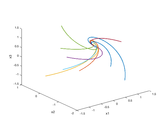
Dynamics of a line attractor network.
Here is the matlab script that made the above figures.
% how the brain keeps the eyes still
% example linear network models

clear; close; clc

% n is number of neurons (you can change this)
n=4;

% the deficiency of rank you want
% point attractors when nullity=0
% line attractors when nullity=1
nullity=0;


dt = 0.001; % time step
tau = 1; % time constant

% construct random matrix of rank N minus nullity (this is M=-I+W)
% and make sure real part of eigenvalus is negative
M = zeros(n,n);
while any(real(eigs(M))>=0)
   M = zeros(n,n);
   for i=1:n-nullity
      M = M + randn(n,1)*randn(1,n);
   end
end
% this makes sure b is in range of M
z = orth(M); b = z*randn(size(z,2),1);

for k=1:10 % number of initial conditions
   x = randn(n,1);
   for i = 1:1e5
      x(:,i+1) = x(:,i)+dt/tau*(M*x(:,i)+b); % M=-I+W
   end

   % only the 2 or 3 first dimensions are plotted
   % (x1, x2) if n=2, (x1, x2, x3) if n>=3
   if n<=2
      plot(x(1,:),x(2,:)); hold on;
      plot(x(1,end),x(2,end),'*','MarkerSize',10);
   else
      plot3(x(1,:),x(2,:),x(3,:),'LineWidth',2); hold on;
      plot3(x(1,end),x(2,end),x(3,end),'*','MarkerSize',10); hold on;
      zlabel('x3')
   end
   xlabel('x1')
   ylabel('x2')
end

You must be logged in to post a comment.